Gravimetry - Importing and processing a gravity survey to compute a Bouguer anomaly
Kaufmann, 2019-2021. Work in progress.
[1]:
import matplotlib.pyplot as plt
import geopandas as gpd
import shapely
from bootsoff.gravity import corrections
Import dataset
[2]:
# importing a built-in dataset. Use bootsoff.gravity.instruments.import_cg6 to import a LRS CG6 file.
from bootsoff.data.gravity import profile as df
The imported dataset is stored as a pandas dataframe.
It includes a geometry field that was programmed in the gravimeter or as been imported from a GNSS receiver
[3]:
df
[3]:
| Station_ID | InstrCorrGrav | StdDev | StdErr | Latitude | Longitude | Ellipsoid Height | InstrHeight | RMS Easting | RMS Elevation | RMS Northing | mask | geometry | |
|---|---|---|---|---|---|---|---|---|---|---|---|---|---|
| datetime | |||||||||||||
| 2019-12-09 06:52:12+00:00 | 1 - BASE_JONCQUOIS_02 | 4296.4051 | 0.1788 | 0.0327 | 50.445443 | 3.958254 | 75.189 | 0.0 | 0.0080 | 0.0204 | 0.0080 | False | POINT (3.95825353703 50.44544330897001) |
| 2019-12-09 06:52:42+00:00 | 1 - BASE_JONCQUOIS_02 | 4296.4063 | 0.0991 | 0.0181 | 50.445443 | 3.958254 | 75.189 | 0.0 | 0.0080 | 0.0204 | 0.0080 | False | POINT (3.95825353703 50.44544330897001) |
| 2019-12-09 06:53:12+00:00 | 1 - BASE_JONCQUOIS_02 | 4296.4068 | 0.1715 | 0.0313 | 50.445443 | 3.958254 | 75.189 | 0.0 | 0.0080 | 0.0204 | 0.0080 | False | POINT (3.95825353703 50.44544330897001) |
| 2019-12-09 07:32:17+00:00 | 1 - 225 | 4297.1063 | 0.2129 | 0.0389 | 50.429907 | 3.688630 | 64.656 | 0.0 | 0.0107 | 0.0238 | 0.0119 | False | POINT (3.68862962157 50.42990663128001) |
| 2019-12-09 07:32:47+00:00 | 1 - 225 | 4297.0937 | 0.1925 | 0.0352 | 50.429907 | 3.688630 | 64.656 | 0.0 | 0.0107 | 0.0238 | 0.0119 | False | POINT (3.68862962157 50.42990663128001) |
| ... | ... | ... | ... | ... | ... | ... | ... | ... | ... | ... | ... | ... | ... |
| 2019-12-19 14:05:25+00:00 | 1 - 317 | 4304.2391 | 0.1454 | 0.0265 | 50.462992 | 3.659931 | 62.741 | 0.0 | 0.0082 | 0.0208 | 0.0068 | False | POINT (3.65993108962 50.46299167397) |
| 2019-12-19 14:05:55+00:00 | 1 - 317 | 4304.2287 | 0.1375 | 0.0251 | 50.462992 | 3.659931 | 62.741 | 0.0 | 0.0082 | 0.0208 | 0.0068 | False | POINT (3.65993108962 50.46299167397) |
| 2019-12-19 14:21:45+00:00 | 1 - 332 | 4304.9160 | 0.1239 | 0.0226 | 50.466507 | 3.650911 | 62.297 | 0.0 | 0.0183 | 0.0537 | 0.0107 | False | POINT (3.6509110203 50.46650696247) |
| 2019-12-19 14:22:15+00:00 | 1 - 332 | 4304.9338 | 0.1479 | 0.0270 | 50.466507 | 3.650911 | 62.297 | 0.0 | 0.0183 | 0.0537 | 0.0107 | False | POINT (3.6509110203 50.46650696247) |
| 2019-12-19 14:22:45+00:00 | 1 - 332 | 4304.9413 | 0.1092 | 0.0199 | 50.466507 | 3.650911 | 62.297 | 0.0 | 0.0183 | 0.0537 | 0.0107 | False | POINT (3.6509110203 50.46650696247) |
959 rows × 13 columns
Define the Base station and get the base point
[4]:
base_station = "1 - BASE_JONCQUOIS_02"
[5]:
base_point = df.query('Station_ID=="%s"' %base_station).iloc[0,:]
Apply corrections
Choose units among mgal, microgal and si
[6]:
units = 'mgal'
Compute corrections
Instrument drift and terrain corrections have not been implemented yet…
[7]:
corrections(df, base_point.name, units=units)
[8]:
list_corr = ['LatCorr', 'AtmCorr', 'AltCorr', 'BougSphCapCorr', 'BougSlabCorr', 'TideCorr']
[9]:
df[list_corr]
[9]:
| LatCorr | AtmCorr | AltCorr | BougSphCapCorr | BougSlabCorr | TideCorr | |
|---|---|---|---|---|---|---|
| datetime | ||||||
| 2019-12-09 06:52:12+00:00 | 0.000000 | 0.000000 | 0.000000 | 0.000000 | 0.000000 | 0.000000 |
| 2019-12-09 06:52:42+00:00 | 0.000000 | 0.000000 | 0.000000 | 0.000000 | 0.000000 | -0.000070 |
| 2019-12-09 06:53:12+00:00 | 0.000000 | 0.000000 | 0.000000 | 0.000000 | 0.000000 | -0.000141 |
| 2019-12-09 07:32:17+00:00 | 1.382146 | -0.001038 | -3.249397 | 1.194199 | 1.179367 | -0.005881 |
| 2019-12-09 07:32:47+00:00 | 1.382146 | -0.001038 | -3.249397 | 1.194199 | 1.179367 | -0.005958 |
| ... | ... | ... | ... | ... | ... | ... |
| 2019-12-19 14:05:25+00:00 | -1.560937 | -0.001226 | -3.840188 | 1.411316 | 1.393787 | 0.020647 |
| 2019-12-19 14:05:55+00:00 | -1.560937 | -0.001226 | -3.840188 | 1.411316 | 1.393787 | 0.020532 |
| 2019-12-19 14:21:45+00:00 | -1.873602 | -0.001270 | -3.977163 | 1.461656 | 1.443501 | 0.016666 |
| 2019-12-19 14:22:15+00:00 | -1.873602 | -0.001270 | -3.977163 | 1.461656 | 1.443501 | 0.016536 |
| 2019-12-19 14:22:45+00:00 | -1.873602 | -0.001270 | -3.977163 | 1.461656 | 1.443501 | 0.016406 |
959 rows × 6 columns
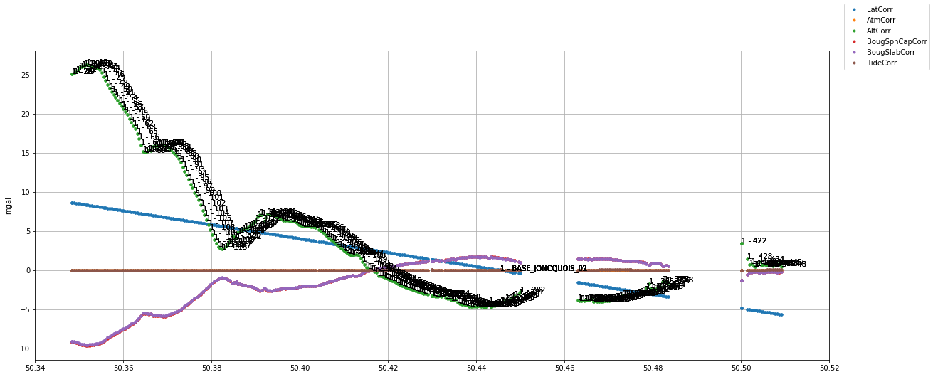
Plot corrections
[10]:
fig, ax = plt.subplots(figsize=(20,8))
lat_lim = [50.34, 50.52]
for i in list_corr:
    ax.plot(df.Latitude, df[i], '.', label=i)
    for idx, row in df.iterrows():
        if (lat_lim[0]<=row.Latitude<=lat_lim[1]) and (i == 'AltCorr'):
            ax.text(row.Latitude, row[i], row['Station_ID'])
ax.set_xlim(lat_lim)
ax.set_ylabel(units)
ax.grid('on')
fig.legend()
[10]:
<matplotlib.legend.Legend at 0x7fe8e0f06100>
Apply corrections to the measurements
[11]:
df['Bouguer'] = df['InstrCorrGrav']+df['LatCorr']+df['AtmCorr']+df['AltCorr']+df['BougSphCapCorr']+df['TideCorr']
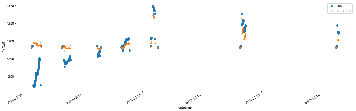
Display the effects of corrections
In time…
[12]:
fig, ax = plt.subplots(nrows=1, figsize=(20,6))
df['InstrCorrGrav'].plot(marker='o', linestyle='none', label='raw')
df['Bouguer'].plot(marker='.', alpha=0.5, linestyle='none', label='corrected')
ax.legend()
ax.set_ylabel('[mGal]')
[12]:
Text(0, 0.5, '[mGal]')
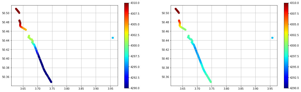
In space…
[13]:
gdf = gpd.GeoDataFrame(df, geometry=df['geometry'].apply(lambda x: shapely.wkt.loads(x)), crs='epsg:4326')
[14]:
fig, ax = plt.subplots(ncols=2, figsize=(20,6))
gdf.plot(column='InstrCorrGrav', ax=ax[0], vmin=4290., vmax=4310, cmap='jet', legend=True)
gdf.plot(column='Bouguer', ax=ax[1], vmin=4290., vmax=4310, cmap='jet', legend=True)
ax[0].grid('on')
ax[1].grid('on')
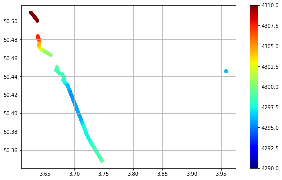
[15]:
fig, ax = plt.subplots(ncols=1, figsize=(10,6))
gdf.plot(column='Bouguer', ax=ax, vmin=4290., vmax=4310, cmap='jet', legend=True)
ax.grid('on')
[ ]: